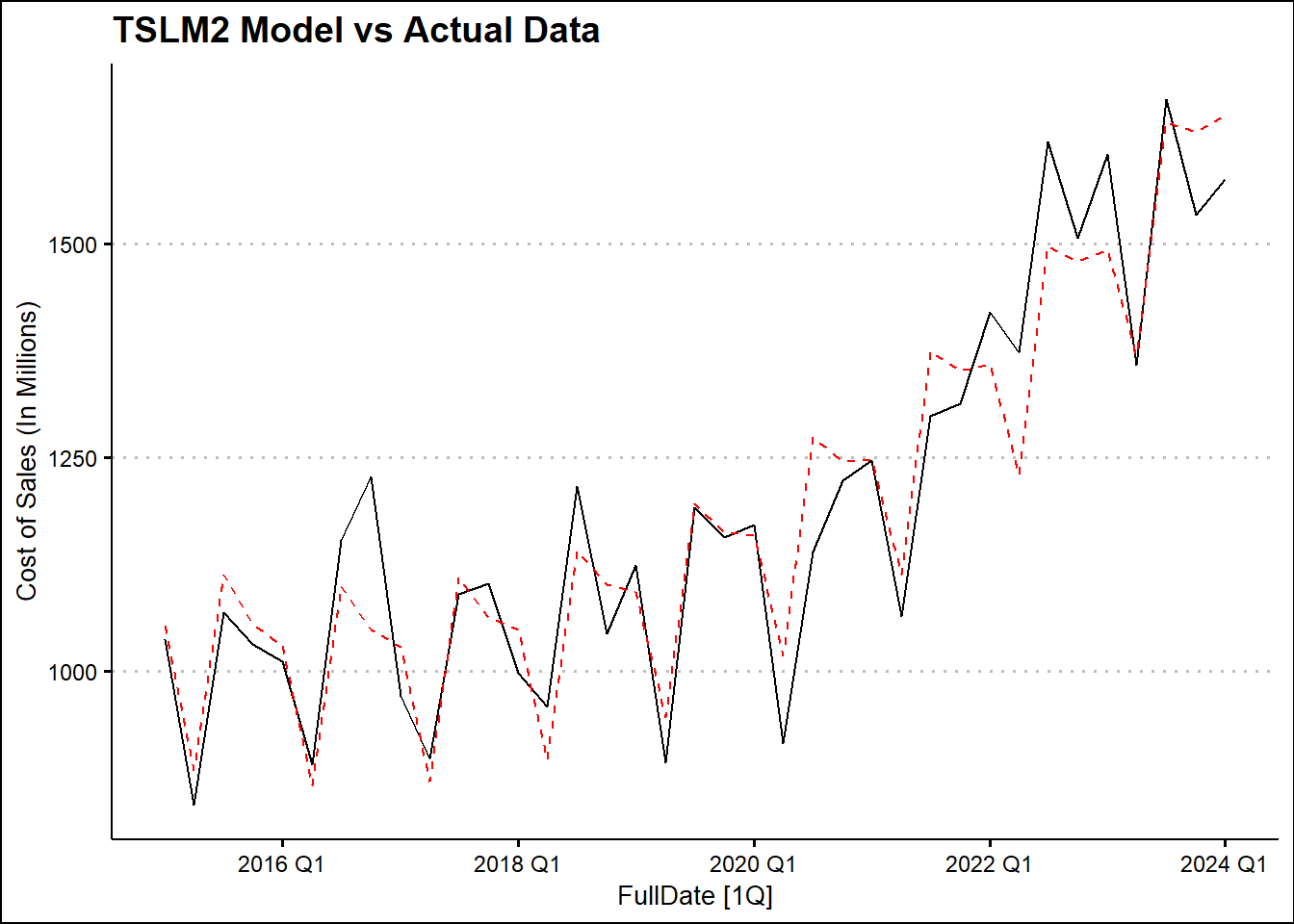
TIME SERIES FORECASTING OF HERSHEY NET SALES & COST OF SALES.

Author

Molly McDade | Ann Gray Perdue | Luke White | John Carl Tagbor

1. Introduction and Company Overview

Hershey Logo

Company Background:

Hershey is a leading company in the confectionery industry, known for producing chocolate, candy, mints, and other snack foods. Founded in 1894 by Milton Hershey, the company is headquartered in Hershey, Pennsylvania.

Hershey’s mission is to bring moments of goodness to people by delivering quality confectionery products. Its key products include the iconic Hershey’s Chocolate Bar, Reese’s Peanut Butter Cups, and Kisses. The company also produces a wide range of snacks, baking products, and beverages.

Hershey operates in both domestic and international markets, with its primary revenue coming from North America. It faces competition from companies like Mars, Nestlé, and Mondelez International.

Motivation for Variables:

Hershey Product Sales

Net Sales:

– Net sales represent the total revenue from Hershey’s products after deductions for discounts, allowances, and returns. This variable is a critical indicator of Hershey’s financial performance as it reflects the company’s ability to generate income from its operations.

– Net sales are influenced by market demand, seasonality, product innovation, and Hershey’s ability to expand into new markets. Understanding future net sales can help predict overall company growth and market share.

Cost of Sales:

– The cost of sales represents the direct costs associated with producing and delivering Hershey’s products. This includes expenses such as raw materials (ex: cocoa, sugar, dairy), labor, and manufacturing overhead.

– Tracking and forecasting the cost of sales is essential to assessing profitability. If costs rise faster than sales, it could squeeze profit margins. Forecasting this variable helps Hershey plan for cost control strategies and maintain operational efficiency.

2. Data and Key Insights

Data Source:

The data for this analysis was sourced directly from Hershey’s quarterly earnings releases, available on the company’s investor relations website at Hershey Investor Relations. The earnings releases provide detailed insights into Hershey’s financial performance, including key metrics such as net sales and cost of sales. These financial statements are publicly available and serve as a reliable source of up-to-date company data.

You can view the individual reports here.

Initial Observations:

Halloween

Seasonality in sales: One notable observation in Hershey’s financial data is the pronounced seasonality of its sales. As outlined in the company’s reports, higher net sales are often recorded during specific periods of the year, particularly around major holidays such as Halloween, Christmas, and Easter. These holidays typically drive increased demand for Hershey’s confectionery products.

Net Sales Growth: Over the last few years, Hershey has experienced a steady growth in net sales, partly due to product innovation, pricing strategies, and the company’s ability to expand into new markets. This upward trend aligns with the broader growth in the snack and confectionery industry.

Cost of Sales Fluctuations: The cost of sales has shown periodic fluctuations, driven by factors such as changes in raw material prices (especially cocoa, sugar, and dairy), supply chain constraints, and rising labor costs. There’s a clear relationship between commodity price volatility and cost of sales, which has implications for Hershey’s overall profitability.

Anomalies: One anomaly noted in the financial data is the impact of the COVID-19 pandemic on sales and costs in early 2020, when demand for certain products temporarily shifted, and supply chains were disrupted.

3. Descriptive Statistics

That data spans Q1 of 2015 to Q4 of 2024. The average net sales over the period under review was $2.16 billion. This is lower than the all time maximum net sales of $3.25 billion which was recorded in Q1 of 2024. This supports the assertion of an upward trend in Net Sales over the period. The script below produces Table 3.1 which displays summary statistics for net sales (in Millions).

library(tidyverse)
library(fpp3)
library(ggthemes)
library(gt)
library(readr)
data <- read_csv("https://raw.githubusercontent.com/lwhite01/Data/main/HersheyData.csv")

data %>% 
  mutate(FullDate = paste(Year, Quarter, sep='Q')) %>% 
  select(Year, Quarter, FullDate, everything()) %>% 
  arrange(FullDate) -> data

###Descriptive Stats of Chosen Variables
des_NS <- tibble(
     Mean = mean(data$`Net Sales (in Millions)`),
     Median = median(data$`Net Sales (in Millions)`),
     Min = min(data$`Net Sales (in Millions)`),
     Max = max(data$`Net Sales (in Millions)`),
) %>% gt() %>% tab_header(
     title = md("**Summary Statistics**"),
     subtitle = "Summary Statistics for Net Sales (in Millions)") %>%
     fmt_number(
          columns = everything(),
          decimals = 0,
          use_seps = TRUE
     ) %>%
tab_options(table.width = px(600))

des_NS

Summary Statistics

Summary Statistics for Net Sales (in Millions)
Mean Median Min Max
2,164 2,033 1,579 3,253


Similarly, Hersheys recorded an average cost of saless of $1.19 billion over the review period. In the last two quarters of the review period, it was more efficient by recording a cost of sales of $1.53 billion in Q4 2023 and $1.58 billion in Q1 2024 compared to a period maximum of $1.67 billion in Q3 2023. The script and Table 3.2 below show summary statistics for cost of sales (in Millions)

des_COS <- tibble(
     Mean = mean(data$`Cost of Sales (In Millions)`),
     Median = median(data$`Cost of Sales (In Millions)`),
     Min = min(data$`Cost of Sales (In Millions)`),
     Max = max(data$`Cost of Sales (In Millions)`),
)%>% gt() %>% tab_header(
     title = md("**Summary Statistics**"),
     subtitle = "Summary Statistics for Cost of Sales (In Millions)") %>%
     fmt_number(
          columns = everything(),
          decimals = 0,
          use_seps = TRUE) %>% 
     tab_options(table.width = px(600))

des_COS

Summary Statistics

Summary Statistics for Cost of Sales (In Millions)
Mean Median Min Max
1,188 1,153 843 1,670


As a result of the high Net Sales of $3.25 billion compared to the cost of sales of $1.58 billion in Q1 2024, it recorded an all time income before tax of $1.68 billion.


Time Series Visualization:

The script below produces a visual of the distribution of Net Sales, Cost of Sales and income before tax over the review period.

ggplot(data, aes(x = FullDate)) +
  geom_line(aes(y = `Net Sales (in Millions)`, color = "Net Sales", group = 1), linewidth = 1) +
  geom_line(aes(y = `Cost of Sales (In Millions)`, color = "Cost of Sales", group = 1), linewidth = 1) +
  geom_line(aes(y = `Income before Income Taxes`, 
                color = "Income Before Taxes", group = 1), linewidth = 1) +
  labs(title = "Net Sales, Cost of Sales, and Income Before Taxes Over Time",
       x = "Time (Year and Quarter)",
       y = "Amount (in Millions)",
       color = "Legend") -> fullPlot

Q1pos <- grep('Q1',data$FullDate)

fullPlot + geom_vline(xintercept = Q1pos, linetype = "dashed", color = "black")

It is evident from the chart above there is an upward trend for all the variables. Seasonality is also evident. Note that black vertical broken lines represent Q1 of each review year. To investigate seasonality and trend further, it is important to consider a decomposition of these elements. These are produced by the scripts below.

# Make time series tsibble

data %>% 
  mutate(FullDate=yearquarter(FullDate)) %>%
  as_tsibble(index=FullDate) %>% 
  mutate(Quarter = factor(quarter(FullDate)))->data_ts

#### NET SALES Decomposition
data_ts %>%
  model(STL=STL(`Net Sales (in Millions)`~trend()+
                  season(), robust=TRUE)) %>%
  components() %>% autoplot()+ theme_classic()

#### COST OF SALES Decomposition
data_ts %>%
  model(STL=STL(`Cost of Sales (In Millions)`~trend()+
                  season(), robust=TRUE)) %>%
  components() %>% autoplot()+ theme_classic()

The charts above confirm the presence of trend and seasonality in the data set. This means it is appropriate to run a time series forecast to predict future net sales and cost of sales.

4. Forecasting

Forecasting Methodology

With the establishment of the data as a suitable time series, the next step would be to select a suitable forecast model. Model Selection: In this project, we used several forecasting models including TSLM (Time Series Linear Model), ETS (Error, Trend, Seasonality), and ARIMA (AutoRegressive Integrated Moving Average) to predict future values of both Net Sales and Cost of Sales. Each model was selected based on its strengths.

  • TSLM was chosen for its ability to model trend and seasonality explicitly, allowing us to incorporate linear relationships over time, including polynomial trends.

  • ETS was used to capture the inherent patterns in the data by decomposing it into error, trend, and seasonality components. This method is highly effective when the data exhibits clear seasonal cycles.

  • ARIMA was selected for its flexibility in handling non-stationary data and its ability to model autocorrelations.

Model Selection

A combination approach (Combo Model) was employed in all instances to improve forecasting accuracy, with weights assigned to different models. In the model selection for Net Sales, a weight of 0.2 for ARIMA and 0.8 for TSLM were applied to balance their strengths. On the other hand, a weight of 0.1 for ETS and 0.9 for TSLM2 was applied to determine a Combo model for Cost of Sales.

The model performance was evaluated using the Winkler Score, a metric used to assess the accuracy of probabilistic forecasts, and various accuracy metrics to select the best-performing models for future predictions.

data_ts %>% filter_index(.~"2022 Q2") -> train
data_ts %>% filter_index("2022 Q3"~"2024 Q1") -> test

###TRAINING THE MODEL TO PREDICT NET SALES & VERIFYING ACCURACY
train %>% model(TSLM=TSLM(`Net Sales (in Millions)`~trend()+season()),
                TSLM2=TSLM(`Net Sales (in Millions)`~trend()+ I(trend()^2) + season()),
                ETS=ETS(`Net Sales (in Millions)`),
                ARIMA=ARIMA(`Net Sales (in Millions)`)) -> fit

# Accuracy of Models

fit %>% forecast(test) %>%
  accuracy(data_ts, list(winkler = winkler_score)) %>% gt() %>% 
     tab_header(title = md("**Winkler Score**")) %>%
  fmt_number(
    columns = winkler,
    decimals = 2,
    use_seps = TRUE
  ) %>%
  tab_options(table.width = px(600))

Winkler Score

.model .type winkler
ARIMA Test 778.60
ETS Test 910.60
TSLM Test 6,855.94
TSLM2 Test 1,037.55
data_ts %>% stretch_tsibble(.init = 20, .step=7) %>%
  model(TSLM=TSLM(`Net Sales (in Millions)`~trend()+season()),
        TSLM2=TSLM(`Net Sales (in Millions)`~trend()+ I(trend()^2) + season()),
        ARIMA=ARIMA(`Net Sales (in Millions)`),
        ETS=ETS(`Net Sales (in Millions)`)) %>% 
  mutate(Combo=0.2*ARIMA+0.8*TSLM2) %>%                 
  forecast(h=7) %>%
  accuracy(data_ts) %>% gt() %>% 
     tab_header(title = md("**Net Sales Model Accuracy**")) %>%
  fmt_number(
    columns = everything(),
    decimals = 2,
    use_seps = TRUE
  ) %>% tab_style(
    style = list(cell_fill(color = "lightblue")),
    locations = cells_body(rows = .model == "Combo"))

Net Sales Model Accuracy

.model .type ME RMSE MAE MPE MAPE MASE RMSSE ACF1
ARIMA Test 180.04 255.56 206.74 6.81 8.08 1.60 1.47 0.57
Combo Test 119.43 217.91 171.50 4.37 6.69 1.33 1.25 0.41
ETS Test 191.76 327.92 261.68 7.54 10.31 2.03 1.88 0.51
TSLM Test 264.26 340.29 275.38 9.85 10.49 2.13 1.95 0.48
TSLM2 Test 104.27 212.07 162.69 3.76 6.34 1.26 1.22 0.37
###TRAINING THE MODEL TO PREDICT COST OF SALES & VERIFYING ACCURACY
train %>% model(TSLM=TSLM(`Cost of Sales (In Millions)`~trend()+season()),
                TSLM2=TSLM(`Cost of Sales (In Millions)`~trend()+ I(trend()^2) + season()),
                ETS=ETS(`Cost of Sales (In Millions)`),
                ARIMA=ARIMA(`Cost of Sales (In Millions)`)) -> fitC

# Accuracy of Models

fitC %>% forecast(test) %>%
  accuracy(data_ts, list(winkler = winkler_score)) %>% gt()%>% 
     tab_header(title = md("**Winkler Score**")) %>%
  fmt_number(
    columns = winkler,
    decimals = 2,
    use_seps = TRUE
  ) %>%
  tab_options(table.width = px(600))

Winkler Score

.model .type winkler
ARIMA Test 869.24
ETS Test 684.06
TSLM Test 1,866.93
TSLM2 Test 386.55
data_ts %>% stretch_tsibble(.init = 20, .step=7) %>%
  model(TSLM=TSLM(`Cost of Sales (In Millions)`~trend()+season()),
        TSLM2=TSLM(`Cost of Sales (In Millions)`~trend()+ I(trend()^2) + season()),
        ARIMA=ARIMA(`Cost of Sales (In Millions)`),
        ETS=ETS(`Cost of Sales (In Millions)`)) %>% 
  mutate(Combo=0.1*ETS+0.9*TSLM2) %>%                 
  forecast(h=7) %>%
  accuracy(data_ts) %>% gt()%>% 
     tab_header(title = md("**Cost of Sales Model Accuracy**")) %>%
  fmt_number(
    columns = everything(),
    decimals = 2,
    use_seps = TRUE
  ) %>% tab_style(
    style = list(cell_fill(color = "lightblue")),
    locations = cells_body(rows = .model == "TSLM2"))

Cost of Sales Model Accuracy

.model .type ME RMSE MAE MPE MAPE MASE RMSSE ACF1
ARIMA Test 111.66 163.22 139.17 8.10 10.11 1.37 1.27 0.61
Combo Test 89.82 158.78 133.85 6.45 9.60 1.32 1.23 0.62
ETS Test 169.64 212.63 173.82 12.27 12.55 1.71 1.65 0.62
TSLM Test 153.93 199.11 164.57 10.63 11.65 1.62 1.54 0.73
TSLM2 Test 80.95 154.60 131.19 5.80 9.39 1.29 1.20 0.62

For validation, cross-validation was used with rolling windows to evaluate model performance across different sections of the data. The accuracy of each model was assessed, and TSLM2 and Combo models were chosen as the most accurate for forecasting.

Finally, forecasts were generated for seven quarters, and prediction intervals were calculated to account for uncertainty. Visualizations were created to compare actual data with the model forecasts, providing a clear assessment of each model’s performance.

Variable 1: Net Sales Forecasting

Using models deemed best based on the winkler score, accuracy, and overall fit, forecasts for the next 7 quarters were created and visualized.

data_ts %>% model(TSLM2=TSLM(`Net Sales (in Millions)`~trend()+ I(trend()^2) + season()),
                  ARIMA=ARIMA(`Net Sales (in Millions)`),
                  ETS=ETS(`Net Sales (in Millions)`)) %>% 
  mutate(Combo=0.2*ARIMA+0.8*TSLM2) -> fit2

fit2 %>% augment() -> resids2

resids2 %>% autoplot(.resid) + theme_clean()

# Plot Combo Model - best here

data_ts %>% autoplot(`Net Sales (in Millions)`) +
  autolayer(resids2 %>% filter(.model=="Combo"),.fitted, 
            lty=2,col="red") +
  theme_clean() +
  labs(title = 'Combo Model vs Actual Data')

# Plot TSLM2 Model

data_ts %>% autoplot(`Net Sales (in Millions)`) +
  autolayer(resids2 %>% filter(.model=="TSLM2"),.fitted, 
            lty=2,col="red") +
  theme_clean() +
  labs(title = 'TSLM2 Model vs Actual Data')

# Plot ARIMA Model

data_ts %>% autoplot(`Net Sales (in Millions)`) +
  autolayer(resids2 %>% filter(.model=="ARIMA"),.fitted, 
            lty=2,col="red") +
  theme_clean() +
  labs(title = 'ARIMA Model vs Actual Data')

fit2 %>% forecast(h=7) %>% hilo(level=95) %>% gt()
.model FullDate Net Sales (in Millions) .mean 95%
TSLM2 2024 Q2 N(2842, 13777) 2841.842 [2611.79150787123, 3071.89195346374]95
TSLM2 2024 Q3 N(3295, 14354) 3295.384 [3060.56348445224, 3530.20449667579]95
TSLM2 2024 Q4 N(3255, 15016) 3255.101 [3014.92834659677, 3495.27304321322]95
TSLM2 2025 Q1 N(3441, 15443) 3440.795 [3197.23407952741, 3684.35675496909]95
TSLM2 2025 Q2 N(3193, 17189) 3193.293 [2936.32967258815, 3450.25559092534]95
TSLM2 2025 Q3 N(3658, 18317) 3657.739 [3392.47380055147, 3923.00399782482]95
TSLM2 2025 Q4 N(3628, 19568) 3628.360 [3354.19087834528, 3902.52834378269]95
ARIMA 2024 Q2 N(2617, 10168) 2617.039 [2419.40126400743, 2814.67609995634]95
ARIMA 2024 Q3 N(3230, 12400) 3230.283 [3012.02702916697, 3448.53835366484]95
ARIMA 2024 Q4 N(2818, 18135) 2818.317 [2554.37555604795, 3082.25856203375]95
ARIMA 2025 Q1 N(3435, 21806) 3434.739 [3145.31214387347, 3724.16680348569]95
ARIMA 2025 Q2 N(2788, 50527) 2787.988 [2347.42187900105, 3228.55505513373]95
ARIMA 2025 Q3 N(3407, 62983) 3407.100 [2915.21721885056, 3898.98201987434]95
ARIMA 2025 Q4 N(2992, 83250) 2992.016 [2426.50641472513, 3557.52526643061]95
ETS 2024 Q2 N(2691, 15809) 2690.656 [2444.2247347798, 2937.08703007662]95
ETS 2024 Q3 N(3126, 23150) 3126.319 [2828.10820168658, 3424.52963252633]95
ETS 2024 Q4 N(2885, 24678) 2884.666 [2576.77019136388, 3192.56110619408]95
ETS 2025 Q1 N(3329, 38996) 3328.761 [2941.71689216728, 3715.80464006609]95
ETS 2025 Q2 N(2816, 62228) 2816.331 [2327.40758502123, 3305.25382437758]95
ETS 2025 Q3 N(3252, 93300) 3251.994 [2653.3204428271, 3850.6670359282]95
ETS 2025 Q4 N(3010, 113975) 3010.340 [2348.6543826324, 3672.02655946795]95
Combo 2024 Q2 N(2797, 11015) 2796.881 [2591.17770991191, 3002.58453194881]95
Combo 2024 Q3 N(3282, 11702) 3282.364 [3070.34601146646, 3494.38145000233]95
Combo 2024 Q4 N(3168, 12833) 3167.744 [2945.71486300093, 3389.77307246341]95
Combo 2025 Q1 N(3440, 13533) 3439.584 [3211.58203089965, 3667.58642616938]95
Combo 2025 Q2 N(3112, 17482) 3112.232 [2853.08767401404, 3371.3759236237]95
Combo 2025 Q3 N(3608, 19383) 3607.611 [3334.74112592587, 3880.48096052014]95
Combo 2025 Q4 N(3501, 21961) 3501.091 [3210.63667766355, 3791.54503626997]95
fit2 %>% select(Combo) %>% forecast(h=7) %>% autoplot(level=95) + 
  autolayer(data_ts, `Net Sales (in Millions)`) +
  theme_clean() +
  labs(title = "Hershey's Projected Net Sales for 2024/2025")

Using Combo model, we plotted the projected Net sales for the net 7 quarters.The forecast of our model shows a decrease in net sales in 2024 Q2 and 2025 Q2 and spikes in holiday-heavy quarters like Q3 & Q4 2024 and Q3 & Q4 2025.

  • Q2 2024: Net Sales $2796.881 M <- Low 2024
  • Q3 2024: Net Sales $3282.364 M <- High 2024
  • Q4 2024: Net Sales $3167.744 M
  • Q1 2025: Net Sales $3439.584 M
  • Q2 2025: Net Sales $3112.232 M <- Low 2025
  • Q3 2025: Net Sales $3607.611 M <- High 2025
  • Q4 2025: Net Sales $3501.091 M

Variable 2: Cost of Sales Forecasting

Similarly, visualizations of the forecast were created for variable 2.

data_ts %>% model(TSLM2=TSLM(`Cost of Sales (In Millions)`~trend()+ I(trend()^2) + season()),
                  ARIMA=ARIMA(`Cost of Sales (In Millions)`),
                  ETS=ETS(`Cost of Sales (In Millions)`)) %>% 
  mutate(Combo=0.1*ETS+0.9*TSLM2) -> fitC2

fitC2 %>% augment() -> residsC2

residsC2 %>% autoplot(.resid) + theme_clean()

# Plot TSLM2 Model - best model here

data_ts %>% autoplot(`Cost of Sales (In Millions)`) +
  autolayer(residsC2 %>% filter(.model=="TSLM2"),.fitted, 
            lty=2,col="red") +
  theme_clean() +
  labs(title = 'TSLM2 Model vs Actual Data')

# Plot ETS Model

data_ts %>% autoplot(`Cost of Sales (In Millions)`) +
  autolayer(residsC2 %>% filter(.model=="ETS"),.fitted, 
            lty=2,col="red") +
  theme_clean() +
  labs(title = 'ETS Model vs Actual Data')

# Plot Combo Model

data_ts %>% autoplot(`Cost of Sales (In Millions)`) +
  autolayer(residsC2 %>% filter(.model=="Combo"),.fitted, 
            lty=2,col="red") +
  theme_clean() +
  labs(title = 'Combo Model vs Actual Data')

fitC2 %>% forecast(h=7) %>% hilo(level=95) %>% gt()
.model FullDate Cost of Sales (In Millions) .mean 95%
TSLM2 2024 Q2 N(1532, 7662) 1532.371 [1360.81323979361, 1703.92967921331]95
TSLM2 2024 Q3 N(1811, 7983) 1811.283 [1636.16728545879, 1986.39853053419]95
TSLM2 2024 Q4 N(1805, 8351) 1805.500 [1626.39319352741, 1984.60663056273]95
TSLM2 2025 Q1 N(1830, 8588) 1830.267 [1648.63322919581, 2011.9012928529]95
TSLM2 2025 Q2 N(1718, 9559) 1717.648 [1526.01981030487, 1909.27619032919]95
TSLM2 2025 Q3 N(2002, 10187) 2002.222 [1804.40229056328, 2200.04118645405]95
TSLM2 2025 Q4 N(2002, 10882) 2002.101 [1797.6417663025, 2206.56029820921]95
ARIMA 2024 Q2 N(1394, 7270) 1394.300 [1227.18914028872, 1561.41087024307]95
ARIMA 2024 Q3 N(1651, 8801) 1650.841 [1466.96575863004, 1834.71685349592]95
ARIMA 2024 Q4 N(1594, 11078) 1594.166 [1387.87482549221, 1800.45626744804]95
ARIMA 2025 Q1 N(1617, 12332) 1617.467 [1399.81087588345, 1835.12250481452]95
ARIMA 2025 Q2 N(1446, 14871) 1445.784 [1206.77149974836, 1684.79619287632]95
ARIMA 2025 Q3 N(1700, 16134) 1700.445 [1451.48751500662, 1949.40292240479]95
ARIMA 2025 Q4 N(1647, 17279) 1646.647 [1389.01125651997, 1904.28318437619]95
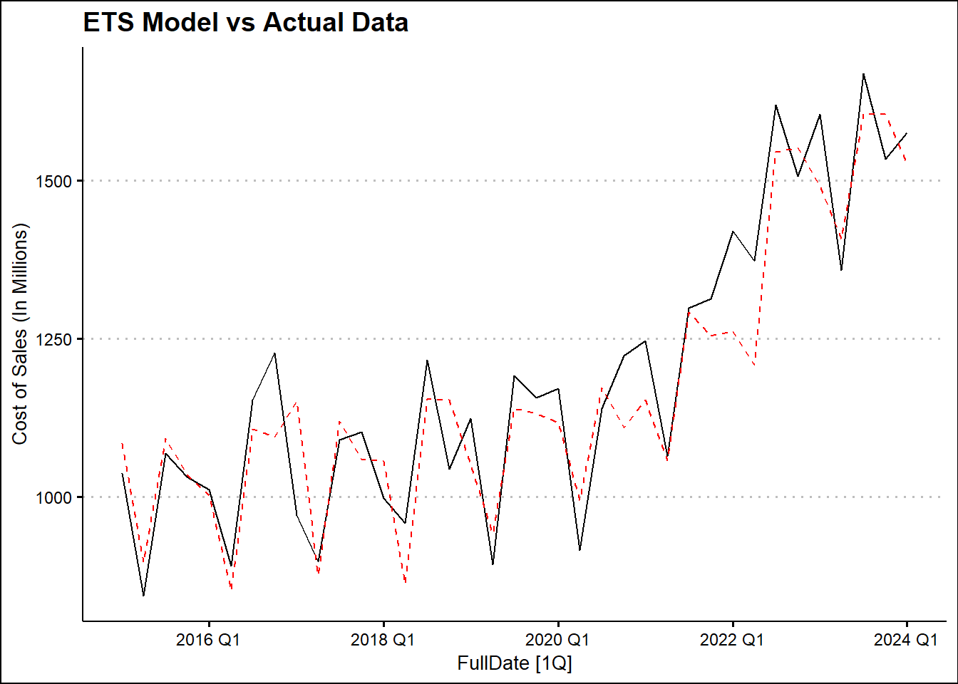
ETS 2024 Q2 N(1402, 10669) 1402.412 [1199.96390438173, 1604.85974076864]95
ETS 2024 Q3 N(1633, 19024) 1632.516 [1362.18076023152, 1902.85052457189]95
ETS 2024 Q4 N(1591, 24491) 1590.645 [1283.91848901443, 1897.37152846756]95
ETS 2025 Q1 N(1560, 29864) 1559.750 [1221.04389072817, 1898.45683977983]95
ETS 2025 Q2 N(1402, 33024) 1402.412 [1046.23808716779, 1758.58555798259]95
ETS 2025 Q3 N(1633, 41430) 1632.516 [1233.57518788673, 2031.45609691668]95
ETS 2025 Q4 N(1591, 46949) 1590.645 [1165.96604408291, 2015.32397339907]95
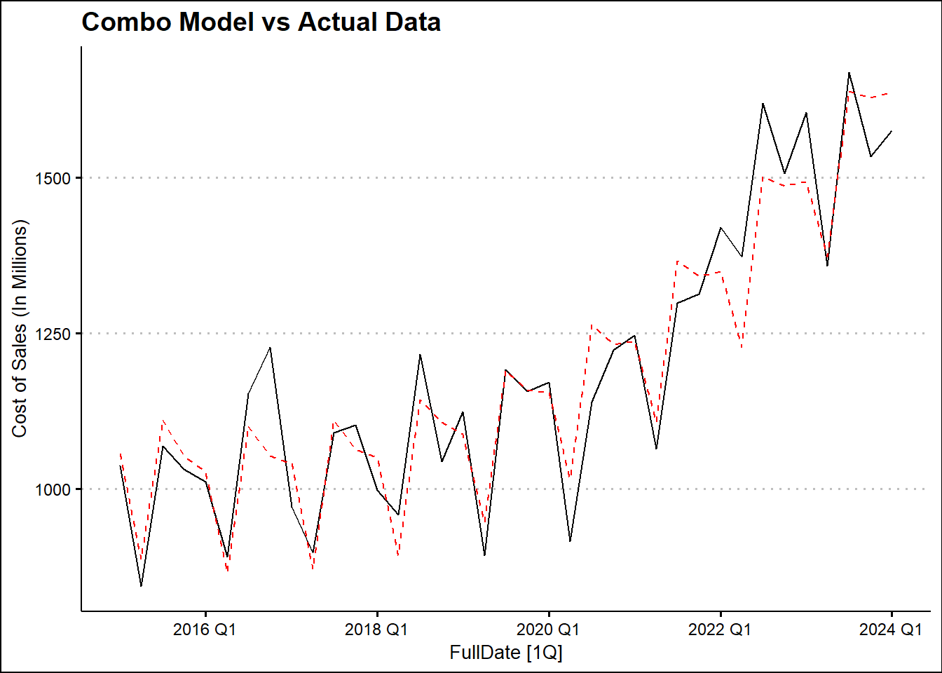
Combo 2024 Q2 N(1519, 7471) 1519.375 [1349.96741497482, 1688.78357664645]95
Combo 2024 Q3 N(1793, 8235) 1793.406 [1615.54634129935, 1971.26602157467]95
Combo 2024 Q4 N(1784, 8841) 1784.014 [1599.72545894822, 1968.3033844811]95
Combo 2025 Q1 N(1803, 9307) 1803.216 [1614.13699703838, 1992.29414585626]95
Combo 2025 Q2 N(1686, 10349) 1686.124 [1486.73492631119, 1885.51383877451]95
Combo 2025 Q3 N(1965, 11297) 1965.251 [1756.92837847104, 2173.57387932489]95
Combo 2025 Q4 N(1961, 12180) 1960.955 [1744.65155841261, 2177.25930139612]95
fitC2 %>% select(TSLM2) %>% forecast(h=7) %>% autoplot(level=95) + 
  autolayer(data_ts, `Cost of Sales (In Millions)`) +
  theme_clean() +
  labs(title = "Hershey's Projected Cost of Sales for 2024/2025")

The forecast of our model shows a decrease in the cost of sales in 2024 Q2 and 2025 Q2 and spikes in the cost of sales in holiday-heavy quarters like Q3 2024 and Q3 2025. This may reflect a relaxed sales cost strategy to compliment relaxed sales in the off holiday season.

  • Q2 2024: Cost of Sales $1532.371 M <-Low 2024
  • Q3 2024: Cost of Sales $1811.283 M <- High 2024
  • Q4 2024: Cost of Sales $1805.500 M
  • Q1 2025: Cost of Sales $1830.267 M
  • Q2 2025: Cost of Sales $1717.648 M <- Low 2025
  • Q3 2025: Cost of Sales $2002.222 M <- High 2024
  • Q4 2025: Cost of Sales $2002.101 M

5. Results and Business Impact

Seasonal Trends in Q3 and Q4

Forecasting Results: In summary, our team discovered that there is a seasonal trend in the net sales and cost of sales of Hershey’s products. Using a Combination model to predict Net Sales TSLM2 model to predict Cost of Sales, both models reflected that sales and costs peak in Q3 and slump in Q2. The seasonal trend reflects a spike of sales in the holiday heavy months in Q3 and Q4, a moderate sales in Q1, and a slump in the summertime months during Q2. This reflects increase chocolate sales and costs of operations that correlate with holidays like Halloween, Christmas, and Valentines Day.

The forecasting values for Net Sales and Cost of Sales:

  • Q2 2024: Cost of Sales $1532.371 M Net Sales $2796.881 M
  • Q3 2024: Cost of Sales $1811.283 M Net Sales $3282.364 M
  • Q4 2024: Cost of Sales $1,805.500 M Net Sales $3167.744 M
  • Q1 2025: Cost of Sales $1830.267 M Net Sales $3439.584 M
  • Q2 2025: Cost of Sales $1717.648 M Net Sales $3112.232 M
  • Q3 2025: Cost of Sales $2002.222 M Net Sales $3607.611 M
  • Q4 2025: Cost of Sales $2002.101 M Net Sales $3501.091 M

Implications for the Company: With this information, we recommend that Hershey continue to decrease its cost of sales of chocolate products in Q2 and increase its cost of sales in Q3 and Q4 to reflect consumer demand. Additionally, we have seen improved sales in Q1, and the cost of sales should be increased to try to increase sales in this period. Alternatively, Hershey could use this information to create a new sales or marketing strategy to increase sales in the dips of Q2.